Alternate Optimal Solutions
Let us solve a small variation of the earlier example, with the same constraints but a slightly different objective:

As before, we add slacks ![]() and
and ![]() , and we solve by the simplex
method, using tableau representation.
, and we solve by the simplex
method, using tableau representation.

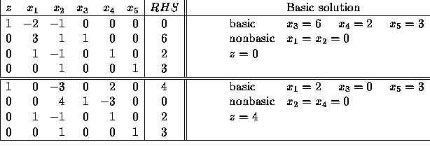
Now Rule 1 shows that this is an optimal solution. Interestingly, the coefficient
of the nonbasic variable ![]() in Row 0 happens to be equal to 0. Going back
to the rationale that allowed us to derive Rule 1, we observe that, if we
increase
in Row 0 happens to be equal to 0. Going back
to the rationale that allowed us to derive Rule 1, we observe that, if we
increase ![]() (from its current value of 0), this will not effect
the value of z. Increasing
(from its current value of 0), this will not effect
the value of z. Increasing ![]() produces changes in the other variables, of course,
through the equations in Rows 1 and 2. In fact, we can use
Rule 2 and pivot to get a different basic solution with the same objective value z=2.
produces changes in the other variables, of course,
through the equations in Rows 1 and 2. In fact, we can use
Rule 2 and pivot to get a different basic solution with the same objective value z=2.

Note that the coefficient of the nonbasic variable ![]() in Row 0 is
equal to 0.
Using
in Row 0 is
equal to 0.
Using ![]() as entering variable and pivoting,
we would recover the previous solution!
as entering variable and pivoting,
we would recover the previous solution!
Degeneracy

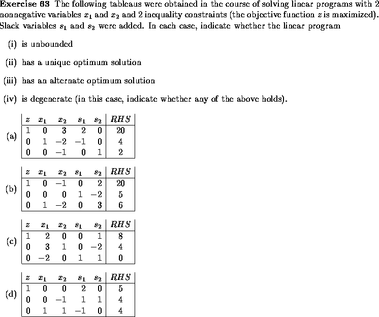
Let us solve this problem using the -by now familiar- simplex method.
In the initial tableau, we can choose ![]() as the entering variable (Rule 1)
and Row 2 as the pivot row (the minimum ratio in Rule 2 is a tie, and ties
are broken arbitrarily). We pivot and this yields the second tableau below.
as the entering variable (Rule 1)
and Row 2 as the pivot row (the minimum ratio in Rule 2 is a tie, and ties
are broken arbitrarily). We pivot and this yields the second tableau below.

Note that this basic solution has a basic variable (namely ![]() ) which
is equal to zero. When this occurs, we say that the basic solution
is degenerate. Should this be of concern? Let us continue the steps
of the simplex method. Rule 1 indicates that
) which
is equal to zero. When this occurs, we say that the basic solution
is degenerate. Should this be of concern? Let us continue the steps
of the simplex method. Rule 1 indicates that ![]() is the entering
variable. Now let us apply Rule 2. The ratios to consider are
is the entering
variable. Now let us apply Rule 2. The ratios to consider are
![]() in Row 1 and
in Row 1 and ![]() in Row 3. The minimum ratio
occurs in Row 1, so let us perform the corresponding pivot.
in Row 3. The minimum ratio
occurs in Row 1, so let us perform the corresponding pivot.

We get exactly the same solution! The only difference is that we have
interchanged the names of a nonbasic variable with that of a degenerate
basic variable ( ![]() and
and ![]() ). Rule 1 tells us the solution is not
optimal, so let us continue the steps of the simplex method. Variable
). Rule 1 tells us the solution is not
optimal, so let us continue the steps of the simplex method. Variable
![]() is the entering variable and the last row wins the minimum ratio
test. After pivoting, we get the tableau:
is the entering variable and the last row wins the minimum ratio
test. After pivoting, we get the tableau:

By Rule 1, this is the optimal solution. So, after all, degeneracy did not prevent the simplex method to find the optimal solution in this example. It just slowed things down a little. Unfortunately, on other examples, degeneracy may lead to cycling, i.e. a sequence of pivots that goes through the same tableaus and repeats itself indefinitely. In theory, cycling can be avoided by choosing the entering variable with smallest index in Rule 1, among all those with a negative coefficient in Row 0, and by breaking ties in the minimum ratio test by choosing the leaving variable with smallest index (this is known as Bland's rule). This rule, although it guaranties that cycling will never occur, turns out to be somewhat inefficient. Actually, in commercial codes, no effort is made to avoid cycling. This may come as a surprise, since degeneracy is a frequent occurence. But there are two reasons for this:
Our example of degeneracy is a 2-variable problem, so you might want to draw the constraint set in the plane and interpret degeneracy graphically.
Unbounded Optimum

Solving by the simplex method, we get:

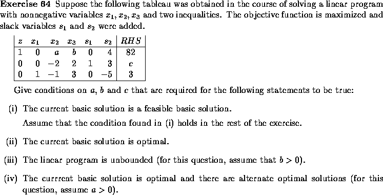
At this stage, Rule 1 chooses ![]() as the entering variable, but
there is no ratio to compute, since there is no positive entry
in the column of
as the entering variable, but
there is no ratio to compute, since there is no positive entry
in the column of ![]() .
As we start increasing
.
As we start increasing ![]() , the value of z increases (from Row 0)
and the values of the basic variables increase as well (from
Rows 1 and 2). There is nothing to stop them going off to infinity.
So the problem is unbounded.
, the value of z increases (from Row 0)
and the values of the basic variables increase as well (from
Rows 1 and 2). There is nothing to stop them going off to infinity.
So the problem is unbounded.
Interpret the steps of the simplex method graphically for this example.
Infeasible Linear Programs
It is easy to construct constraints that have no solution. The simplex method is able to identify such cases. We do not discuss it here. The interested reader is referred to Winston, for example.
Properties of Linear Programs
There are three possible outcomes for a linear program: it is infeasible, it has an unbounded optimum or it has an optimal solution.
If there is an optimal solution, there is a basic optimal solution. Remember that the number of basic variables in a basic solution is equal to the number of constraints of the problem, say m. So, even if the total number of variables, say n, is greater than m, at most m of these variables can have a positive value in an optimal basic solution.


Answer:
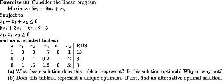
(a)
The solution is ![]() ,
, ![]() , objective 15. It is
optimal since cost row is all at least 0.
, objective 15. It is
optimal since cost row is all at least 0.
(b)
It is not unique (since ![]() has reduced cost 0 but is not
basic). Alternative found by pivoting in
has reduced cost 0 but is not
basic). Alternative found by pivoting in ![]() (question could have
asked for details on such a pivot) for solution
(question could have
asked for details on such a pivot) for solution ![]() ,
, ![]() , objective 15.
, objective 15.