I think the clearest way to present the scenario approach is to give an extended example. This example is similar to many faced in business every day: any aspect of inventory control or raw material stockpiling can be seen in the following.
We are a computer manufacturer. After meeting this periods demand, we have capacity for producing 1500 computer, each of which can be either a high-end or a low-end machine. These computers will be used to help meet demand next period. In addition, we we have the capacity to produce 2000 computers next period after we see next periods demand. Profit on each low-end sold next period is $200; each high-end gives $250. It costs $25 to store a low-end for one period and $50 to store a high-end. Any produced low-end machine that remains unsold after the next period results in a loss of $100; any unsold high-end gives a loss of $150.
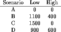
Demand next period is uncertain, but can be modeled as being one of the following four scenarios:

What should we produce this period in order to handle demand next period?
First, note that if we know the future, the production process is an easy linear program. For scenario A, we get the linear program:
L1: First period low-end production
H1: First period high-end production
L2: Second period low-end production
H2: Second period high-end production
LS: Sales of low-end
HS: Sales of high-end
LW: Unsold (wasted) low end
HW: Unsold (wasted) high end

max -25 l1 - 50 h1 + 200 ls + 150 hs - 100 lw - 150 hw
st
(1) l1 + l2 - lw - ls = 0
(2) ls < 1000
(3) h1 + h2 - hw - hs = 0
(4) hs < 1000
(5) l2 + h2 < 2000
(6) l1 + h1 < 1500
end
The other scenarios are identical with a change in demand constraints (2) and (4). Each of these can be solved (by inspection) to give the following optimal solutions:

But, of course, we don't know the future: we need to decide on L1 and H1 before we know what the future is. Now many people have heuristic ways of aggregating these choices: they use expected demand, or take the ``expected value'' of the above decisions. It is possible, however, to create a single linear program that takes into account all of the scenarios.
As with any model with a probabilistic aspect, you must carefully decide what you want to optimize. One natural choice is to optimize the expected value. The following linear program does just that:
L1: First period low-end production
H1: First period high-end production
L2A, L2B, L2C, L2D: Second period low-end production in scenario
                    A, B, C, and D.
H2A, H2B, H2C, H2D: Second period high-end production in scenario
                    A, B, C, and D
LSA, LSB, LSC, LSD: Sales of low-end in each scenario
HSA, HSB, HSC, HSD: Sales of high-end in each scenario
LWA, LWB, LWC, LWD: Unsold (wasted) low end in each scenario
HWA, HWB, HWC, HWD: Unsold (wasted) high end in each scenario

max -25 l1 - 50 h1
+40 lsa + 50hsa-20 lwa-30hwa
+60 lsb + 75hsb-30 lwb-45lwb
+80 lsc + 100hsc-40 lwc-60lwc
+20 lsd + 25hsd-10 lwd-15lwd
st
l1+l2a-lwa - lsa = 0
lsa < 1000
h1+h2a-hwa - hsa = 0
hsa < 1000
l2a+h2a < 2000
l1+l2b-lwb - lsb = 0
lsb < 1100
h1+h2b-hwb - hsb = 0
hsb < 2400
l2b+h2b < 2000
l1+l2c-lwc - lsc = 0
lsc < 2000
h1+h2c-hwc - hsc = 0
hsc < 1500
l2c+h2c < 2000
l1+l2d-lwd - lsd = 0
lsd < 2000
h1+h2d-hwd - hsd = 0
hsd < 2600
l2d+h2d < 2000
l1+h1 < 1500
end
First, the expected profit from, say, LSA, is 200 (the profit) times 0.2 (the probability). Second, there is no L1A, L1B and so on since the first decision must be made without information about the set.
The optimal solution to this model is:
        L1      1000.000000
        H1       500.000000
       LSA      1000.000000
       HSA      1000.000000
       LSB      1100.000000
       HSB      2400.000000
       LSC      2000.000000
       HSC      1500.000000
       LSD      1000.000000
       HSD      2500.000000
       H2A       500.000000
       L2B       100.000000
       H2B      1900.000000
       L2C      1000.000000
       H2C      1000.000000
       H2D      2000.000000
with the rest of the variables having value 0. The optimal first period decision doesn't match up the the best decision for any scenario!
The value for this solution is $678,500. If we knew the future, we could make the optimal choice for each possibility. The expect value in such a situation is $694,500. The value we could then place on learning the future is $16,000. We would be willing to pay up to $16,000 to learn next period's demand before this period's production decision.
Expected value is not the only possible objective. For instance, it may be that we are unwilling to take a loss in any possible future. Our goal could then be to maximize expected value subject to never having a loss. This would have the same objective, but we would add constraints of the form:
-25 l1 - 50 h1 + 200 lsa + 150 hsa - 100 lwa - 150 hwa >= 0
Or the objective might be to maximize the minimum profit we make. This and many other objectives can be handled by this linear program.