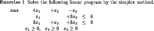
For simplicity, in this course we solve ``by hand'' only the case
where the constraints are of the form ![]() and the
right-hand-sides are nonnegative.
We will explain the steps of the simplex method while we progress
through an example.
and the
right-hand-sides are nonnegative.
We will explain the steps of the simplex method while we progress
through an example.
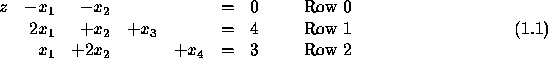
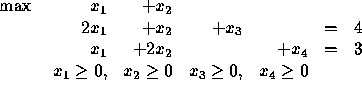
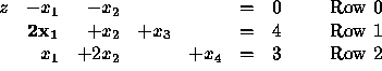
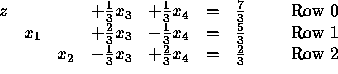
First, we convert the problem into standard form by adding slack
variables ![]() and
and ![]() .
.
Let z denote the objective function value. Here, ![]() or,
equivalently,
or,
equivalently,
![]()
Putting this equation together with the constraints, we get the following system of linear equations.
Our goal is to maximize z, while satisfying these equations and,
in addition, ![]() ,
, ![]() ,
, ![]() ,
, ![]() .
.
Note that the equations are already in the form that we expect at
the last step of the Gauss-Jordan procedure. Namely, the equations
are solved in terms of the nonbasic variables ![]() ,
, ![]() .
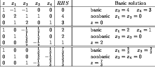
The variables (other than the special variable z) which appear
in only one equation are the basic variables. Here the basic
variables are
.
The variables (other than the special variable z) which appear
in only one equation are the basic variables. Here the basic
variables are ![]() and
and ![]() . A basic solution is obtained
from the system of equations by setting the nonbasic variables
to zero. Here this yields
. A basic solution is obtained
from the system of equations by setting the nonbasic variables
to zero. Here this yields
![]()
Is this an optimal solution or can we increase z? (Our goal)
By looking at Row 0 above, we see that we can increase z by increasing
![]() or
or ![]() . This is because these variables have a negative coefficient
in Row 0. If all coefficients in Row 0 had been nonnegative, we could have
concluded that the current basic solution is optimum, since there would be no
way to increase z (remember that all variables
. This is because these variables have a negative coefficient
in Row 0. If all coefficients in Row 0 had been nonnegative, we could have
concluded that the current basic solution is optimum, since there would be no
way to increase z (remember that all variables ![]() must remain
must remain ![]() ).
We have just discovered the first rule of the simplex method.
).
We have just discovered the first rule of the simplex method.
Rule 1
If all variables have a nonnegative coefficient in Row 0, the current
basic solution is optimal.
Otherwise, pick a variable ![]() with a negative coefficient in Row 0.
with a negative coefficient in Row 0.
The variable chosen by Rule 1 is called the entering variable.
Here let us choose, say, ![]() as our entering variable. It really does not
matter which variable we choose as long as it has a negative coefficient
in Row 0.
The idea is to pivot in order to make the nonbasic
variable
as our entering variable. It really does not
matter which variable we choose as long as it has a negative coefficient
in Row 0.
The idea is to pivot in order to make the nonbasic
variable ![]() become a basic variable. In the process, some
basic variable will become nonbasic (the leaving variable).
This change of basis is done using
the Gauss-Jordan procedure. What is needed next is to choose the
pivot element. It will be found using Rule 2 of the simplex
method. In order to
better understand the rationale behing this second rule, let us try
both possible pivots and see why only one is acceptable.
become a basic variable. In the process, some
basic variable will become nonbasic (the leaving variable).
This change of basis is done using
the Gauss-Jordan procedure. What is needed next is to choose the
pivot element. It will be found using Rule 2 of the simplex
method. In order to
better understand the rationale behing this second rule, let us try
both possible pivots and see why only one is acceptable.
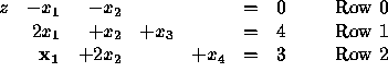
First, try the pivot element in Row 1.
This yields
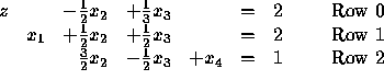
with basic solution
![]()
Now, try the pivot element in Row 2.
This yields
with basic solution
![]()
Which pivot should we choose? The first one, of course, since the second
yields an infeasible basic solution! Indeed, remember that we must
keep all variables ![]() . With the second pivot, we get
. With the second pivot, we get ![]() which
is infeasible. How could we have known this ahead of time,
before actually performing the pivots? The answer is, by comparing the ratios
which
is infeasible. How could we have known this ahead of time,
before actually performing the pivots? The answer is, by comparing the ratios
![]() in Rows 1 and 2 of (1.1).
Here we get
in Rows 1 and 2 of (1.1).
Here we get ![]() in Row 1 and
in Row 1 and ![]() in Row 2. If you pivot in a row with minimum ratio, you will
end up with a feasible basic solution (i.e. you will not introduce negative
entries in the Right Hand Side), whereas if you pivot in a row with a
ratio which is not minimum you will always end up with an infeasible
basic solution. Just simple algebra! A negative pivot element would not be
good either, for the
same reason. We have just discovered the second rule of the simplex method.
in Row 2. If you pivot in a row with minimum ratio, you will
end up with a feasible basic solution (i.e. you will not introduce negative
entries in the Right Hand Side), whereas if you pivot in a row with a
ratio which is not minimum you will always end up with an infeasible
basic solution. Just simple algebra! A negative pivot element would not be
good either, for the
same reason. We have just discovered the second rule of the simplex method.
Rule 2
For each Row i, ![]() , where there is a strictly positive
``entering variable coefficient'', compute the ratio of the
Right Hand Side to the ``entering variable coefficient''. Choose
the pivot row as being the one with MINIMUM ratio.
, where there is a strictly positive
``entering variable coefficient'', compute the ratio of the
Right Hand Side to the ``entering variable coefficient''. Choose
the pivot row as being the one with MINIMUM ratio.
Once you have idendified the pivot element by Rule 2, you perform a Gauss-Jordan pivot. This gives you a new basic solution. Is it an optimal solution? This question is addressed by Rule 1, so we have closed the loop. The simplex method iterates between Rules 1, 2 and pivoting until Rule 1 guarantees that the current basic solution is optimal. That's all there is to the simplex method.
After our first pivot, we obtained the following system of equations.
with basic solution
![]()
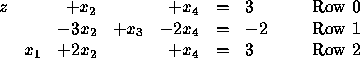
Is this solution optimal? No, Rule 1 tells us to choose ![]() as
entering variable. Where should we pivot? Rule 2 tells us to pivot in
Row 2, since the ratios are
as
entering variable. Where should we pivot? Rule 2 tells us to pivot in
Row 2, since the ratios are ![]() for Row 1, and
for Row 1, and
![]() for Row 2, and the minimum occurs in Row 2.
So we pivot on
for Row 2, and the minimum occurs in Row 2.
So we pivot on ![]() in the above system of equations. This yields
in the above system of equations. This yields
with basic solution ![]()
Now Rule 1 tells us that this basic solution is optimal, since there are no more negative entries in Row 0.
All the above computations can be represented very compactly in tableau form.
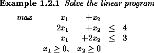
Since the above example has only two variables, it is interesting to
interpret the steps of the simplex method graphically.
See Figure 1.1. The simplex method starts in the corner
point ![]() with z=0. Then it discovers that z can
increase by increasing, say,
with z=0. Then it discovers that z can
increase by increasing, say, ![]() . Since we keep
. Since we keep ![]() , this means
we move along the
, this means
we move along the ![]() axis. How far can we go? Only until we hit
a constraint: if we went any further, the solution would become infeasible.
That's exactly what Rule 2 of the simplex method does: the minimum
ratio rule identifies the first constraint that will be encountered.
And when the constraint is reached, its slack
axis. How far can we go? Only until we hit
a constraint: if we went any further, the solution would become infeasible.
That's exactly what Rule 2 of the simplex method does: the minimum
ratio rule identifies the first constraint that will be encountered.
And when the constraint is reached, its slack ![]() becomes zero.
So, after the first pivot, we are at the point
becomes zero.
So, after the first pivot, we are at the point ![]() .
Rule 1 discovers that z can be increased by increasing
.
Rule 1 discovers that z can be increased by increasing ![]() while
keeping
while
keeping ![]() . This means that we move along the boundary of the
feasible region
. This means that we move along the boundary of the
feasible region ![]() until we reach another constraint!
After pivoting, we reach the optimal point
until we reach another constraint!
After pivoting, we reach the optimal point
![]() .
.
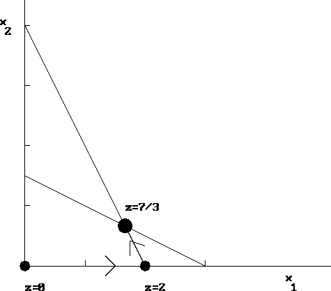
Figure 1.1: Graphical Interpretation