How do we handle both equality and inequality constraints in (P)? Let (P) be:
Maximize f(x)
Subject to
![]()
![]()
![]()
![]()
![]()
![]()
If you have a program with ![]() constraints, convert it into
constraints, convert it into ![]() by
multiplying by -1. Also convert a minimization to a maximization.
by
multiplying by -1. Also convert a minimization to a maximization.
The Lagrangian is
![]()
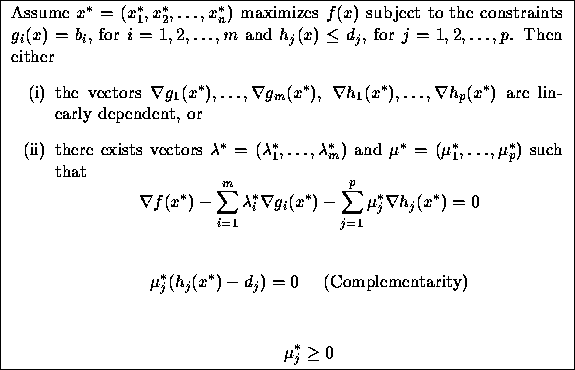
The fundamental result is the following:

In this course, we will not concern ourselves with Case (i).
We will only look for candidate solutions ![]() for which we
can find
for which we
can find ![]() and
and ![]() satisfying the equations in
Case (ii) above.
satisfying the equations in
Case (ii) above.
In general, to solve these equations, you begin with complementarity and note
that either ![]() must be zero or
must be zero or ![]() . Based on the
various possibilities, you come up with one or more candidate
solutions. If there is an optimal solution, then one of your
candidates will be it.
. Based on the
various possibilities, you come up with one or more candidate
solutions. If there is an optimal solution, then one of your
candidates will be it.
The above conditions are called the Kuhn-Tucker (or Karush-Kuhn-Tucker) conditions. Why do they make sense?
For ![]() optimal, some of the inequalities will be tight and some
not. Those not tight can be ignored (and will have corresponding
price
optimal, some of the inequalities will be tight and some
not. Those not tight can be ignored (and will have corresponding
price ![]() ). Those that are tight can be treated as equalities which
leads to the previous Lagrangian stuff. So
). Those that are tight can be treated as equalities which
leads to the previous Lagrangian stuff. So
![]()
forces either the price ![]() to be 0 or the constraint to be
tight.
to be 0 or the constraint to be
tight.


Economic Interpretation
The economic interpretation is essentially the same as the equality
case. If the right hand side of a constraint
is changed by a small amount ![]() ,
then the optimal objective changes by
,
then the optimal objective changes by ![]() ,
where
,
where ![]() is the optimal Lagrange multiplier corresponding
to that constraint. Note that if the
constraint is not tight then the objective does not change (since then
is the optimal Lagrange multiplier corresponding
to that constraint. Note that if the
constraint is not tight then the objective does not change (since then
![]() ).
).
Handling Nonnegativity
A special type of constraint is nonnegativity. If you have a
constraint ![]() , you can write this as
, you can write this as ![]() and use the
above result. This constraint would get a Lagrange multiplier of its own,
and would be treated just like every other constraint.
and use the
above result. This constraint would get a Lagrange multiplier of its own,
and would be treated just like every other constraint.
An alternative is to treat nonnegativity implicitly. If ![]() must be
nonnegative:
must be
nonnegative:
![]()

Sufficiency of conditions
The Karush-Kuhn-Tucker conditions give us candidate
optimal solutions ![]() . When are these conditions sufficient
for optimality? That is, given
. When are these conditions sufficient
for optimality? That is, given ![]() with
with ![]() and
and ![]() satisfying the KKT conditions, when can we be certain that it is an
optimal solution?
satisfying the KKT conditions, when can we be certain that it is an
optimal solution?
The most general condition available is:
While it is straightforward to determine if the objective is concave by computing its Hessian matrix, it is not so easy to tell if the feasible region is convex. A useful condition is as follows:
The feasible region is convex if all of the ![]() are linear and
all of the
are linear and
all of the ![]() are convex.
are convex.
If this condition is satisfied, then any point that satisfies the KKT conditions gives a point that maximizes f(x) subject to the constraints.

Review of Optimality Conditions.
The following reviews what we have learned so far:
Single Variable (Unconstrained)
Solve f'(x) = 0 to get candidate ![]() .
.
If ![]() then
then ![]() is a local min.
is a local min.
![]() then
then ![]() is a local max.
is a local max.
If f(x) is convex then a local min is a global min.
f(x) is concave then a local max is a global max.
Multiple Variable (Unconstrained)
Solve ![]() to get candidate
to get candidate ![]() .
.
If ![]() is positive definite then
is positive definite then ![]() is a local min.
is a local min.
![]() is negative definite
is negative definite ![]() is a local max.
is a local max.
If f(x) is convex then a local min is a global min.
f(x) is concave then a local max is a global max.
Multiple Variable (Equality constrained)
Form Lagrangian ![]()
Solve ![]() to get candidate
to get candidate ![]() (and
(and
![]() ).
).
Best ![]() is optimum if optimum exists.
is optimum if optimum exists.
Multiple Variable (Equality and Inequality constrained)
Put into standard form (maximize and ![]() constraints)
constraints)
Form Lagrangian ![]()
Solve
![]()
![]()
![]()
![]()
![]()
to get candidates ![]() (and
(and ![]() ,
, ![]() ).
).
Best ![]() is optimum if optimum exists.
is optimum if optimum exists.
Any ![]() is optimum if f(x) concave,
is optimum if f(x) concave, ![]() convex,
convex,
![]() linear.
linear.