The values ![]() have an important economic interpretation:
If the right hand side
have an important economic interpretation:
If the right hand side ![]() of Constraint i is increased by
of Constraint i is increased by
![]() , then the optimum objective value increases
by approximately
, then the optimum objective value increases
by approximately ![]() .
.
In particular, consider the problem
Maximize p(x)
subject to
g(x)=b,
where p(x) is a profit to maximize and b is a limited
amount of resource. Then, the optimum Lagrange multiplier ![]() is the marginal value of the resource. Equivalently,
if b were increased by
is the marginal value of the resource. Equivalently,
if b were increased by ![]() , profit would increase by
, profit would increase by ![]() .
This is an important result to remember. It will be used repeatedly
in your Managerial Economics course.
.
This is an important result to remember. It will be used repeatedly
in your Managerial Economics course.
Similarly, if
Minimize c(x)
subject to
d(x)=b,
represents the minimum cost c(x) of meeting some demand b,
the optimum Lagrange multiplier ![]() is the marginal cost of
meeting the demand.
is the marginal cost of
meeting the demand.
In Example 4.1.2
Minimize ![]()
subject to
![]() ,
,
if we change the right hand side from 1 to 1.05 (i.e.
![]() ), then the optimum objective function value
goes from
), then the optimum objective function value
goes from ![]() to roughly
to roughly
![]()
If instead the right hand side became 0.98, our estimate of the optimum objective function value would be
![]()
![]()
![]()
![]()
![]()
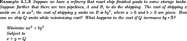
The first two constraints give ![]() , which leads to
, which leads to
![]()
and cost of ![]() . The Hessian matrix
. The Hessian matrix
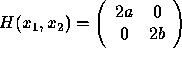 is positive definite since a;SPMgt;0 and b;SPMgt;0. So this solution minimizes
cost, given a,b,Q.
is positive definite since a;SPMgt;0 and b;SPMgt;0. So this solution minimizes
cost, given a,b,Q.
If Q increases by r%, then the RHS of the constraint
increases by ![]() and the minimum cost increases by
and the minimum cost increases by
![]() . That is, the minimum cost increases
by 2r%.
. That is, the minimum cost increases
by 2r%.
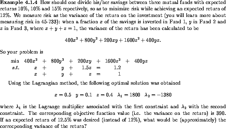
Since ![]() , the variance would increase by
, the variance would increase by
![]()
So the answer is 390+90=480.