The single input two-output or two input-one output problems are easy to analyze graphically. The previous numerical example is now solved graphically. (An assumption of constant returns to scale is made and explained in detail later.) The analysis of the efficiency for bank B looks like the following:
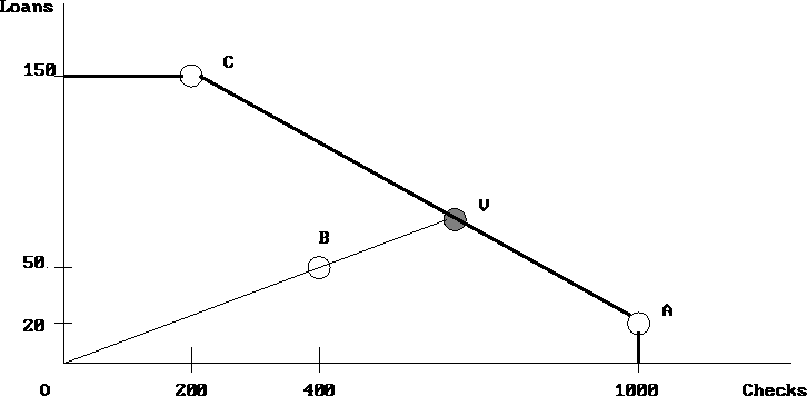
If it is assumed that convex combinations of banks are allowed, then the line segment connecting banks A and C shows the possibilities of virtual outputs that can be formed from these two banks. Similar segments can be drawn between A and B along with B and C. Since the segment AC lies beyond the segments AB and BC, this means that a convex combination of A and C will create the most outputs for a given set of inputs.
This line is called the efficiency frontier. The efficiency frontier defines the maximum combinations of outputs that can be produced for a given set of inputs.
Since bank B lies below the efficiency frontier, it is inefficient. Its efficiency can be determined by comparing it to a virtual bank formed from bank A and bank C. The virtual player, called V, is approximately 54% of bank A and 46% of bank C. (This can be determined by an application of the lever law. Pull out a ruler and measure the lengths of AV, CV, and AC. The percentage of bank C is then AV/AC and the percentage of bank A is CV/AC.)
The efficiency of bank B is then calculated by finding the fraction of inputs that bank V would need to produce as many outputs as bank B. This is easily calculated by looking at the line from the origin, O, to V. The efficiency of player B is OB/OV which is approximately 63%. This figure also shows that banks A and C are efficient since they lie on the efficiency frontier. In other words, any virtual bank formed for analyzing banks A and C will lie on banks A and C respectively. Therefore since the efficiency is calculated as the ratio of OA/OV or OA/OV, banks A and C will have efficiency scores equal to 1.0.
The graphical method is useful in this simple two dimensional example but gets much harder in higher dimensions. The normal method of evaluating the efficiency of bank B is by using an linear programming formulation of DEA.
Since this problem uses a constant input value of 10 for all of the banks, it avoids the complications caused by allowing different returns to scale. Returns to scale refers to increasing or decreasing efficiency based on size. For example, a manufacturer can achieve certain economies of scale by producing a thousand circuit boards at a time rather than one at a time - it might be only 100 times as hard as producing one at a time. This is an example of increasing returns to scale (IRS.)
On the other hand, the manufacturer might find it more than a trillion times as difficult to produce a trillion circuit boards at a time though because of storage problems and limits on the worldwide copper supply. This range of production illustrates decreasing returns to scale (DRS.) Combining the two extreme ranges would necessitate variable returns to scale (VRS.)
Constant Returns to Scale (CRS) means that the producers are able to linearly scale the inputs and outputs without increasing or decreasing efficiency. This is a significant assumption. The assumption of CRS may be valid over limited ranges but its use must be justified. As an aside, CRS tends to lower the efficiency scores while VRS tends to raise efficiency scores.