Data Envelopment Analysis, is a linear programming procedure for a frontier analysis of inputs and outputs. DEA assigns a score of 1 to a unit only when comparisons with other relevant units do not provide evidence of inefficiency in the use of any input or output. DEA assigns an efficiency score less than one to (relatively) inefficient units. A score less than one means that a linear combination of other units from the sample could produce the same vector of outputs using a smaller vector of inputs. The score reflects the radial distance from the estimated production frontier to the DMU under consideration.
There are a number of equivalent formulations for DEA. The most direct formulation of the exposition I gave above is as follows:
Let ![]() be the vector of inputs into DMU i. Let
be the vector of inputs into DMU i. Let ![]() be the
corresponding vector of outputs. Let
be the
corresponding vector of outputs. Let ![]() be the inputs into a DMU
for which we want to determine its efficiency and
be the inputs into a DMU
for which we want to determine its efficiency and ![]() be the
outputs. So the X's and the Y's are the data.
The measure of efficiency for
be the
outputs. So the X's and the Y's are the data.
The measure of efficiency for ![]() is given by the following
linear program:
is given by the following
linear program:

where ![]() is the weight given to DMU i in its efforts to
dominate DMU 0 and
is the weight given to DMU i in its efforts to
dominate DMU 0 and ![]() is the efficiency of DMU 0. So the
is the efficiency of DMU 0. So the
![]() 's and
's and ![]() are the variables. Since DMU 0 appears
on the left hand side of the equations as well,
the optimal
are the variables. Since DMU 0 appears
on the left hand side of the equations as well,
the optimal ![]() cannot possibly be more than 1. When we solve
this linear program, we get a number of things:
cannot possibly be more than 1. When we solve
this linear program, we get a number of things:
DEA assumes that the inputs and outputs have been correctly identified. Usually, as the number of inputs and outputs increase, more DMUs tend to get an efficiency rating of 1 as they become too specialized to be evaluated with respect to other units. On the other hand, if there are too few inputs and outputs, more DMUs tend to be comparable. In any study, it is important to focus on correctly specifying inputs and outputs.

The linear programs for evaluating the 3 DMUs are given by:
min THETA
st
5L1+8L2+7L3 - 5THETA <= 0
14L1+15L2+12L3 - 14THETA <= 0
9L1+5L2+4L3 >= 9
4L1+7L2+9L3 >= 4
16L1+10L2+13L3 >= 16
L1, L2, L3 >= 0
min THETA
st
5L1+8L2+7L3 - 8THETA <= 0
14L1+15L2+12L3 - 15THETA <= 0
9L1+5L2+4L3 >= 5
4L1+7L2+9L3 >= 7
16L1+10L2+13L3 >= 10
L1, L2, L3 >= 0
min THETA
st
5L1+8L2+7L3 - 7THETA <= 0
14L1+15L2+12L3 - 12THETA <= 0
9L1+5L2+4L3 >= 4
4L1+7L2+9L3 >= 9
16L1+10L2+13L3 >= 13
L1, L2, L3 >= 0
The solution to each of these is as follows:
Adjustable Cells
                  Final    Reduced  Objective  Allowable   Allowable
 Cell  Name       Value       Cost Coefficien   Increase    Decrease
 $B$10 theta          1          0          1      1E+30           1
 $B$11 L1             1          0          0 0.92857142 0.619047619
 $B$12 L2             0 0.24285714          0      1E+30 0.242857143
 $B$13 L3             0          0          0 0.36710963 0.412698413

Constraints
                  Final      Shadow   Constraint Allowable  Allowable
 Cell  Name       Value       Price   R.H. Side   Increase   Decrease
 $B$16 IN1    -0.103473           0           0      1E+30          0
 $B$17 IN2    -0.289724 -0.07142857           0          0      1E+30
 $B$18 OUT1           9 0.085714286           9          0          0
 $B$19 OUT2           4 0.057142857           4          0          0
 $B$20 OUT3          16           0          16          0      1E+30
Adjustable Cells
                   Final    Reduced  Objective  Allowable   Allowable
 Cell  Name        Value       Cost Coefficien   Increase    Decrease
 $B$10 theta 0.773333333          0         1       1E+30           1
 $B$11 L1    0.261538462          0         0 0.866666667 0.577777778
 $B$12 L2              0 0.22666667         0       1E+30 0.226666667
 $B$13 L3    0.661538462          0         0 0.342635659 0.385185185

Constraints
                  Final     Shadow  Constraint   Allowable   Allowable
 Cell  Name       Value      Price   R.H. Side    Increase    Decrease
 $B$16 IN1  -0.24820512          0           0      1E+30  0.248205128
 $B$17 IN2    -0.452651 -0.0666667           0 0.46538461        1E+30
 $B$18 OUT1           5       0.08           5      10.75  0.655826558
 $B$19 OUT2           7  0.0533333           7 1.05676855   3.41509434
 $B$20 OUT3 12.78461538          0          10 2.78461538        1E+30
Adjustable Cells
                  Final     Reduced   Objective  Allowable    Allowable
 Cell  Name       Value        Cost  Coefficien   Increase     Decrease
 $B$10 theta          1           0           1      1E+30            1
 $B$11 L1             0           0           0 1.08333333  0.722222222
 $B$12 L2             0 0.283333333           0      1E+30  0.283333333
 $B$13 L3             1           0           0 0.42829457  0.481481481

Constraints
                  Final      Shadow Constraint  Allowable  Allowable
 Cell  Name       Value       Price  R.H. Side   Increase   Decrease
 $B$16 IN1    -0.559375           0          0      1E+30          0
 $B$17 IN2    -0.741096 -0.08333333          0          0      1E+30
 $B$18 OUT1           4         0.1          4      16.25          0
 $B$19 OUT2           9 0.066666667          9          0          0
 $B$20 OUT3          13           0         13          0      1E+30
Note that DMUs 1 and 3 are overall efficient and DMU 2 is inefficient with an efficiency rating of 0.773333.
Hence the efficient levels of inputs and outputs for DMU 2 are given by:
![]()

Note that the outputs are at least as much as the outputs currently produced by DMU 2 and inputs are at most as big as the 0.773333 times the inputs of DMU 2. This can be used in two different ways: The inefficient DMU should target to cut down inputs to equal at most the efficient levels. Alternatively, an equivalent statement can be made by finding a set of efficient levels of inputs and outputs by dividing the levels obtained by the efficiency of DMU 2. This focus can then be used to set targets primarily for outputs rather than reduction of inputs.
Alternate Formulation
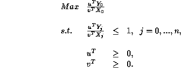
There is another, probably more common formulation, that provides the same information. We can think of DEA as providing a price on each of the inputs and a value for each of the outputs. The efficiency of a DMU is simply the ratio of the inputs to the outputs, and is constrained to be no more than 1. The prices and values have nothing to do with real prices and values: they are an artificial construct. The goal is to find a set of prices and values that puts the target DMU in the best possible light. The goal, then is to

Here, the variables are the u's and the v's. They are vectors of prices and values respectively.
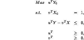
This fractional program can be equivalently stated
as the following linear programming problem
(where Y and X are matrices with columns ![]() and
and ![]() respectively).
respectively).

We denote this linear program by (D). Let us compare it with the one introduced earlier, which we denote by (P):

To fix ideas, let us write out explicitely these two formulations for DMU 2, say, in our example.
Formulation (P) for DMU 2:
min                     THETA
st
-5 L1 - 8 L2 - 7 L3 + 8 THETA >= 0
-14L1 -15 L2 -12 L3 + 15THETA >= 0
 9 L1 + 5 L2 + 4 L3           >= 5
 4 L1 + 7 L2 + 9 L3           >= 7
 16L1 +10 L2 +13 L3           >= 10
L1>=0, L2>=0, L3>=0
Formulation (D) for DMU 2:
max             5 U1 + 7 U2 + 10 U3
st
- 5 V1 - 14V2 + 9 U1 + 4 U2 + 16 U3 <= 0
- 8 V1 - 15V2 + 5 U1 + 7 U2 + 12 U3 <= 0
- 7 V1 - 12V2 + 4 U1 + 9 U2 + 13 U3 <= 0
  8 V1 + 15V2                        = 1
    V1>=0, V2>=0, U1>=0, U2>=0,  U3>=0
Formulations (P) and (D) are dual linear programs! These two formulations actually give the same information. You can read the solution to one from the shadow prices of the other. We will not discuss linear programming duality in this course. You can learn about it in some of the OR electives.
