Cuts for Special Structure

 

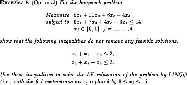
Gomory cuts have the property that they can be generated for any integer program. Their weakness is their downfall: they do not seem to cut off much more than the linear programming solution in practice. An alternative approach is to generate cuts that are specially designed for the particular application. We saw that in a simple form in the lockbox problem, where we used the constraints because they were stronger than . In this section, we examine the symmetric traveling salesperson problem.

Recall that there is no good, compact formulation for the TSP. Earlier, we generated a formulation as follows:

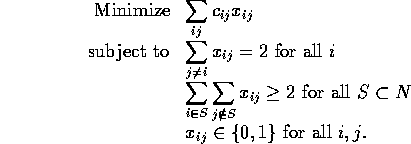
Recall that in the second set of constraints (called subtour elimination constraints) there are many, many constraints. One approach is to initially ignore these constraints and simply solve the problem over the first set of constraints. Suppose we have a six node problem as shown in Figure 6.

  
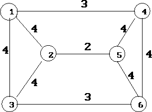
Figure 6: Six node traveling salesperson problem

This problem can be formulated as follows (ignoring subtour constraints):

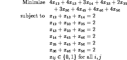
Solving the LP relaxation in LINGO gives:

model
  min = 4 * x12 + 4 * x13 + 3 * x14 + 4 * x23 + 2 * x25 + 3 * x36
      + 4 * x45 + 4 * x46 + 4 * x56;
  x12 + x13 + x14 = 2;
  x12 + x23 + x25 = 2;
  x13 + x23 + x36 = 2;
  x14 + x45 + x46 = 2;
  x25 + x45 + x56 = 2;
  x36 + x46 + x56 = 2;
  @bnd(0,x12,1); @bnd(0,x13,1); @bnd(0,x14,1); 
  @bnd(0,x23,1); @bnd(0,x25,1); @bnd(0,x36,1); 
  @bnd(0,x45,1); @bnd(0,x46,1); @bnd(0,x56,1);
end
 
OPTIMUM FOUND AT STEP          9
SOLUTION OBJECTIVE VALUE =     20.00

           VARIABLE           VALUE        REDUCED COST
                X12       0.5000000           0.0000000E+00
                X13       0.5000000           0.0000000E+00
                X14        1.000000           -1.000000
                X23       0.5000000           0.0000000E+00
                X25        1.000000           -2.000000
                X36        1.000000           -1.000000
                X45       0.5000000           0.0000000E+00
                X46       0.5000000           0.0000000E+00
                X56       0.5000000           0.0000000E+00

This solution, while obviously not a tour, actually satisfies all of the subtour elimination constraints. At this point we have three choices:

1. We can do branch and bound on our current linear program, or
2. We can apply Gomory cuts to the resulting tableau, or
3. We can try to find other classes of cuts to use.

In fact, for the traveling salesperson problem, there are a number of other classes of cuts to use. These cuts look at different sets of arcs and try to say something about how a tour can use them. For instance, look at the set of arcs in Figure 7.

  
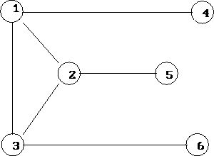
Figure 7: Arc Set for Comb Inequality

It is fairly easy to convince yourself that no tour can use more than 4 of these arcs. This is an example of a broad class of inequalities called comb inequalities. This means that the inequality stating that the sum of the x values on these arcs is less than or equal to 4 is a valid inequality (it does not remove any feasible solution to the integer program). Our solution, however, has 4.5 units on those arcs. Therefore, we can add a constraint to get the following formulation and result:

model
  min = 4 * x12 + 4 * x13 + 3 * x14 + 4 * x23 + 2 * x25 + 3 * x36
      + 4 * x45 + 4 * x46 + 4 * x56;
  x12 + x13 + x14 = 2;
  x12 + x23 + x25 = 2;
  x13 + x23 + x36 = 2;
  x14 + x45 + x46 = 2;
  x25 + x45 + x56 = 2;
  x36 + x46 + x56 = 2;
  x12 + x13 + x23 + x14 + x25 + x36 < 4;
  @bnd(0,x12,1); @bnd(0,x13,1); @bnd(0,x14,1); 
  @bnd(0,x23,1); @bnd(0,x25,1); @bnd(0,x36,1); 
  @bnd(0,x45,1); @bnd(0,x46,1); @bnd(0,x56,1);
end

OPTIMUM FOUND AT STEP         11
SOLUTION OBJECTIVE VALUE =     21.00

           VARIABLE           VALUE        REDUCED COST
                X12       0.0000000E+00       0.0000000E+00
                X13        1.000000           0.0000000E+00
                X14        1.000000           0.0000000E+00
                X23        1.000000           0.0000000E+00
                X25        1.000000           -1.000000
                X36       0.0000000E+00       0.0000000E+00
                X45       0.0000000E+00       0.0000000E+00
                X46        1.000000           0.0000000E+00
                X56        1.000000           0.0000000E+00

So, we have the optimal solution.

This method, perhaps combined with branch and bound if the solution is still fractional after all known inequalities are examined, has proven to be a very practical and robust method for solving medium-sized TSPs. Futhermore, many classes of inequalities are known for other combinatorial optimization problems. This approach, seriously studied only for the last ten years or so, has greatly increased the size and type of instances that can be effectively solved to optimality.