Suppose we have a problem:
Maximize ![]()
subject to
![]()
If we ignore the constraint, we get the solution ![]() ,
which is too large for the constraint. Let us penalize ourselves
,
which is too large for the constraint. Let us penalize ourselves
![]() for making the constraint too big. We end up with a
function
for making the constraint too big. We end up with a
function
![]()
This function is called the Lagrangian of the problem. The main
idea is to adjust ![]() so that we use exactly the right amount of
the resource.
so that we use exactly the right amount of
the resource.
![]() leads to (2,1).
leads to (2,1).
![]() leads to (3/2,0) which uses too little of the
resource.
leads to (3/2,0) which uses too little of the
resource.
![]() gives (5/3, 1/3) and the constraint is satisfied
exactly.
gives (5/3, 1/3) and the constraint is satisfied
exactly.
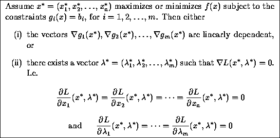
We now explore this idea more formally. Given a nonlinear program (P) with equality constraints:
Minimize (or maximize) f(x)
subject to
![]()
![]()
![]()
![]()
a solution can be found using the Lagrangian:
![]()
(Note: this can also be written ![]() ).
).
Each ![]() gives the price associated with constraint
i.
gives the price associated with constraint
i.
The reason L is of interest is the following:

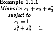
Of course, Case (i) above cannot occur when there is only one constraint. The following example shows how it might occur.

It is easy to check directly that the minimum is acheived
at ![]() . The associated Lagrangian is
. The associated Lagrangian is
![]()
Observe that
![]()
and consequently ![]() does not
vanish at the optimal solution. The reason for this is the following.
Let
does not
vanish at the optimal solution. The reason for this is the following.
Let ![]() and
and ![]() denote
the left hand sides of the constraints. Then
denote
the left hand sides of the constraints. Then ![]() and
and ![]() are linearly dependent vectors.
So Case (i) occurs here!
are linearly dependent vectors.
So Case (i) occurs here!
Nevertheless, Case (i) will not concern us in this course. When solving
optimization problems with equality constraints, we will only look
for solutions ![]() that satisfy Case (ii).
that satisfy Case (ii).
Note that the equation
![]()
is nothing more than
![]()
In other words, taking the partials with respect to ![]() does
nothing more than return the original constraints.
does
nothing more than return the original constraints.
Once we have found candidate solutions ![]() , it is not always
easy to figure out whether they correspond to a minimum, a maximum
or neither. The following situation is one when we can conclude.
If f(x) is concave and all of the
, it is not always
easy to figure out whether they correspond to a minimum, a maximum
or neither. The following situation is one when we can conclude.
If f(x) is concave and all of the
![]() are linear, then any feasible
are linear, then any feasible ![]() with a corresponding
with a corresponding
![]() making
making ![]() maximizes f(x)
subject to the constraints.
Similarly, if f(x) is convex and each
maximizes f(x)
subject to the constraints.
Similarly, if f(x) is convex and each ![]() is linear, then any
is linear, then any
![]() with a
with a ![]() making
making ![]() minimizes
f(x) subject to the constraints.
minimizes
f(x) subject to the constraints.
![]()
![]()
![]()
![]()
Now, the first two equations imply ![]() . Substituting into the
final equation gives the solution
. Substituting into the
final equation gives the solution ![]() ,
, ![]() and
and ![]() , with function value 2/3.
, with function value 2/3.
Since ![]() is convex (its Hessian matrix
is convex (its Hessian matrix
 is positive definite) and
 ![]() is a linear
function, the above solution minimizes
is a linear
function, the above solution minimizes ![]() subject
to the constraint.
subject
to the constraint.