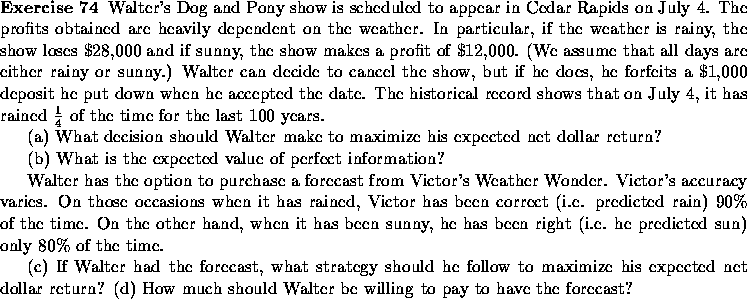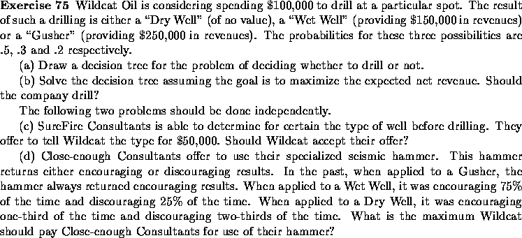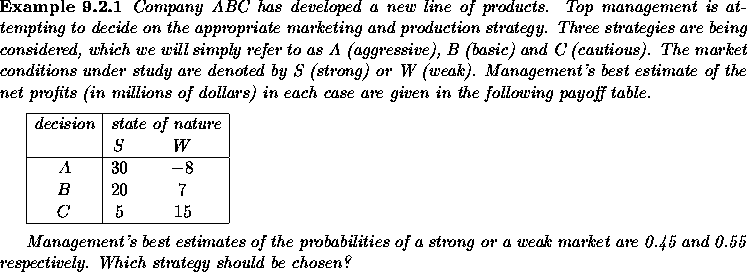

Using the approach introduced earlier, we can compute the expected return for each decision and select the best one, just as we did for the newsboy problem.

The optimal decision is to select B.
A convenient way to represent this problem is through the use of decision trees, as in Figure 9.1. A square node will represent a point at which a decision must been made, and each line leading from a square will represent a possible decision. A circular node will represent situations where the outcome is uncertain, and each line leading from a circle will represent a possible outcome.
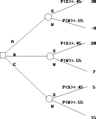
Figure 9.1: Decision Tree for the ABC Company
Using a decision tree to find the optimal decision is called solving the tree. To solve a decision tree, one works backwards. This is called folding back the tree. First, the terminal branches are folded back by calculating an expected value for each terminal node. See Figure 9.2.
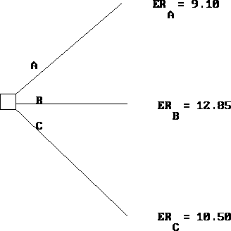
Figure 9.2: Reduced Decision Tree for the ABC Company
Management now faces the simple problem of choosing the alternative that yields the highest expected terminal value. So, a decision tree provides another, more graphic, way of viewing the same problem. Exactly the same information is utilized, and the same calculations are made.
Sensitivity Analysis
The expected return of strategy A is
![]()
or, equivalently,
![]()
Thus, this expected return is a linear function of the probability that market conditions will be strong. Similarly
![]()
We can plot these three linear functions on the same set of axes (see Figure 9.3).
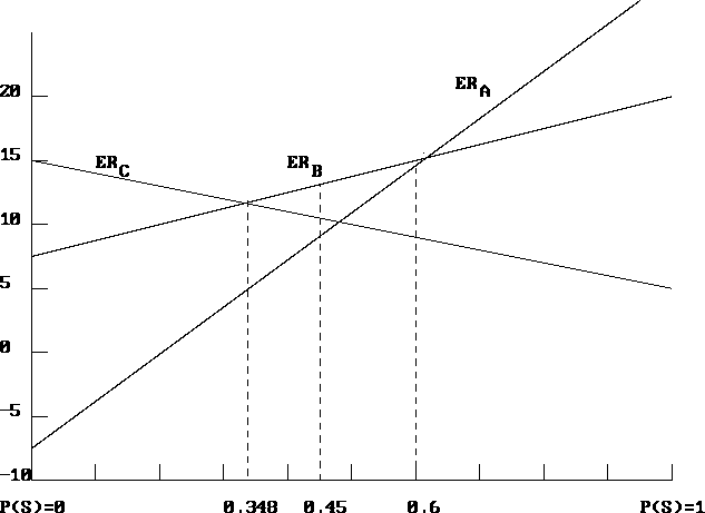
Figure 9.3: Expected Return as a function of P(S)
This diagram shows that Company ABC should select the basic strategy (strategy B) as long as the probability of a strong market demand is between P(S)=0.348 and P(S)= 0.6. This is reassuring, since the optimal decision in this case is not very sensitive to an accurate estimation of P(S). However, if P(S) falls below 0.348, it becomes optimal to choose the cautious strategy C, whereas if P(S) is above 0.6, the agressive strategy A becomes optimal.
Sequential Decisions

Let us construct the decision tree for this sequential decision problem. See Figure 9.4. It is important to note that the tree is created in the chronological order in which information becomes available. Here, the sequence of events is
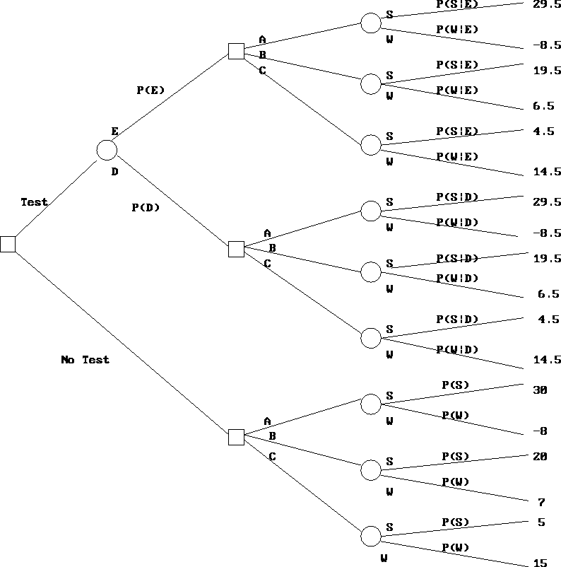
Figure 9.4: Test versus No-Test Decision Tree
The leftmost node correspond to the decision to test or not to test. Moving along the ``Test'' branch, the next node to the right is circular, since it corresponds to an uncertain event. There are two possible results. Either the test is encouraging (E), or it is discouraging (D). The probabilities of these two outcomes are P(E) and P(D) respectively. How does one compute these probabilities?
We need some fundamental results about probabilities. Refer to 45-733 for additional material. The information we are given is conditional. Given S, the probability of E is 60% and the probability of D is 40%. Similarly, we are told that, given W, the probability of E is 30% and the probability of D is 70%. We denote these conditional probabilities as follows
![]()
In addition, we know P(S)=0.45 and P(W)=0.55. This is all the
information we need to compute P(E) and P(D). Indeed, for events
![]() that partition the space of possible outcomes
and an event T,
one has
that partition the space of possible outcomes
and an event T,
one has
![]()
Here, this gives

and

As we continue to move to the right of the decision tree, the next nodes
are square, corresponding to the three marketing and production strategies.
Still further to the right are circular nodes corresponding to the
uncertain market conditions: either weak or strong. The probability of
these two events is now conditional on the outcome of earlier
uncertain events, namely the result of the market reseach study, when
such a study was performed. This means that we need to compute the
following conditional probabilities: ![]() and P(W|D). These quantities are computed using the formula
and P(W|D). These quantities are computed using the formula
![]()
which is valid for any two events R and T. Here, we get
![]()
Similarly,
![]()
Now, we are ready to solve the decision tree. As earlier, this is done by folding back. See Figures 9.5, 9.6 and 9.7. You fold back a circular node by calculating the expected returns. You fold back a square node by selecting the decision that yields the highest expected return. The expected return when the market research study is performed is 12.96 million dollars, which is greater than the expected return when no study is performed. So the study should be undertaken.
As a final note, let us compare the expected value of the study (denoted by EVSI, which stands for expected value of sample information) to the expected value of perfect information EVPI.
EVSI is computed without incorporating the cost of the study. So
![]()
whereas
![]()
We see that the market research study is not very effective. If it were, the value of EVSI would be much closer to EVPI. Yet, its value is greater than its cost, so it is worth performing.

Answer:
(a)
(b) The value is 10, for an expected profit of $10,000. He should buy the painting immediately.
(c) With probability 2/3, the painting will be sold on the first day, so should be bought immediately. With probability 1/3(2/3) it will be sold on the second day, so should be bought after one day. Finally, with probability 1/3(1/3) it will not be sold on the first two days, so should be bought after two days. The value of this is 2/3(10)+1/3(2/3)20+1/3(1/3)25 = 13.89. The EVPI is therefore $3,889.

