Let f be a function of one variable
defined for all x in some domain D. A global
maximum of f is a point ![]() in D such that
in D such that ![]() for all x in D.
for all x in D.
For a constant ![]() ,
the neighborhood
,
the neighborhood ![]() of a point
of a point ![]() is the set of all
points x such that
is the set of all
points x such that ![]() .
A point
.
A point ![]() is a local maximum of f if there exists
is a local maximum of f if there exists
![]() such that
such that ![]() for all x in
for all x in
![]() where f(x) is defined.
where f(x) is defined.

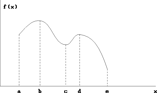
Figure 2.1: local maxima and minima
Similarly one can define local and global minima. In Figure 2.1, the function f is defined for x in domain [ a , e ]. Points b and d are local maxima and b is a global maximum, whereas a, c, and e are local minima and e is a global minimum.
Finding extrema
Extrema, whether they are local or global, can occur in three places:
1. at the boundary of the domain,
2. at a point without a derivative, or
3. at a point ![]() with
with ![]() .
.
The last case is particularly important. So we discuss it
further.
Let f be differentiable in a neighborhood of ![]() . If
. If
![]() is a local extremum of f, then
is a local extremum of f, then ![]() .
Conversely, if
.
Conversely, if ![]() , three possibilities may arise:
, three possibilities may arise:
![]() is a local maximum,
is a local maximum, ![]() is a local minimum, or neither!!!
To decide between these three possibilities, one may use the
second derivative.
Let f be twice differentiable in a neighborhood of
is a local minimum, or neither!!!
To decide between these three possibilities, one may use the
second derivative.
Let f be twice differentiable in a neighborhood of ![]() .
.
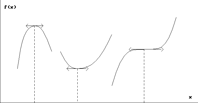
Figure 2.2 illustrates these three possibilities.

Figure 2.2: ![]() ,
, ![]() and one of the possibilities
with
and one of the possibilities
with ![]()

The revenue at price x is
![]()
We compute the derivative of g and set it to 0.
![]()
Since f(x);SPMgt;0 for all x, setting g'(x)=0 implies 1-0.2x=0. So x=5. This is the only possible local optimum. To determine whether it is a maximum or a minimum, we compute the second derivative.
![]()
Putting in x=5 shows g''(x);SPMlt;0, so this is a maximum: the oil cartel maximizes its revenue by pricing gasoline at $5 per gallon.

We must first calculate the holding cost (cost of stockpiling). If each order period begins with Q cases and ends with zero cases, and if usage is more or less constant, then the average stock level is Q/2. This means that the average holding cost is hQ/2.
Since each order of Q cases lasts Q/d weeks, the average ordering
cost per week is ![]() Thus the average total cost per week is
Thus the average total cost per week is
![]()
To find Q that minimizes cost, we set to zero the derivative with respect to Q.
![]()
This implies that the optimal order quantity is
![]()
This is the classical economic order quantity (EOQ) model for inventory management. (You will learn when the EOQ model is appropriate and when to use other inventory models in 45-765).
