OR in the Press – Mike Trick's Operations Research Blog

Touring the Rio Olympics

I’m a sportswriter who is bound for the Olympics, and I’m writing an article about maximizing the number of events I see in a particular day.

I thought the input of a mathematician with expertise in these matters would be helpful to the story.

This was an interesting start to day a month ago. I received this email from New York Times reporter Victor Mather via University of Waterloo prof Bill Cook. Victor had contacted Bill since Bill is the world’s foremost expert on the Traveling Salesman Problem (he has a must-read book aimed at the general public called In Pursuit of the Traveling Salesman: Mathematics at the Limits of Computation). The TSP involves visiting a number of sites while traveling the minimum distance. While Victor’s task will have some aspects of the TSP, there are scheduling aspects that I work on so Bill recommended me (thanks Bill!).

Victor’s plan was to visit as many Olympic events in Rio as he could in a single day. This was part of a competition with another reporter, Sarah Lyall. Victor decided to optimize his day; Sarah would simply go where her heart took her. Who would see more events?

Victor initially just wanted to talk about how optimization would work (or at least he made it seem so) but I knew from the first moment that I would be optimizing his day if he would let me. He let me. He agreed to get me data, and I would formulate and run a model that would find his best schedule.

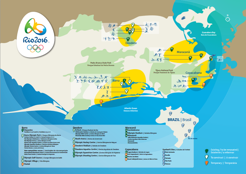
On the day they chose (Monday, August 15), there were 20 events being held. The map shows that the venues are all spread out across Rio (a dense, somewhat chaotic, city not known for its transportation infrastructure). So we would have to worry about travel distance. Victor provided an initial distance matrix, with times in minutes (OLY times). As we will see, this matrix must have been created by someone who had a few too many caipirinhas on Copacabana Beach: it did not exactly match reality.

So far the problem does look like a TSP: just minimize the distance to see 20 sites. The TSP on 20 sites is pretty trivial (see a previous blog post for how hard solving TSPs are in practice) so simply seeing the sites would be quite straightforward. However, not surprisingly Victor actually wanted to see the events happening. For that, we needed a schedule of the events, which Victor promptly provided:

Badminton 8:30 am – 10:30 am // 5:30 pm -7
Basketball 2:15 pm – 4:15 pm// 7 pm -9 pm // 10:30 pm – midnite
Beach Volleyball 4 p.m.-6 p.m. // 11pm – 1 am
Boxing 11 am-1:30 pm, 5 pm – 7:30 pm
Canoeing 9 am – 10:30 am
Cycling: 10 a.m. – 11 am /// 4 pm – 5:30
Diving 3:15 pm -4:30
Equestrian 10 am- 11 am
Field Hockey 10 am – 11:30 am // 12:30 –2 // 6-7:30 pm // 8:30 pm -10
Gymnastics 2 pm -3 pm
Handball: 9:30 am- 11 am// 11:30 – 1pm //2:40 -4 //4:40 – 6 pm // 7:50 – 9:10 pm // 9:50 pm -11:10
Open water Swimming 9 am – 10 am
Sailing 1 pm – 2 pm
Synchronized swimming: 11 am- 12:30
Table tennis 10 am -11 am // 3pm -4:30 // 7:30pm – 9
Track 9:30 am -11:30 am // 8:15pm -10 pm
Volleyball 9:30 am- 10:30 am // 11:30 – 12:30 // 3pm – 4 pm // 5 pm – 6 pm // 8:30 pm -9:30 // 1030 pm -11:30
Water polo 2:10 pm – 3 pm // 3:30 -4:20 //6:20 -7:10 // 7:40 – 8:30
Weightlifting 3:30 – 4:30 pm // 7 pm- 8 pm
Wrestling 10 am – noon // 4 pm- 6 pm

Many events have multiple sessions: Victor only had to see one session at each event, and decided that staying for 15 minutes was enough to declare that he had “seen” the event. It is these “time windows” that make the problem hard(er).

With the data, I promptly sat down and modeled the problem as an mixed-integer program. I had variables for the order in which the events were seen, the time of arrival at each event, and the session seen for each event (the first, second, third or so on). There were constraints to force the result to be a path through the sites (we didn’t worry about where Victor started or ended: travel to and from his hotel was not a concern) and constraints to ensure that when he showed up at an event, there was sufficient time for him to see the event before moving on.

The objective was primarily to see as many events as possible. With this data, it is possible to see all 20 events. At this point, if you would like to see the value of optimization, you might give it a try: can you see all 20 events just by looking at the data? I can’t!

But there may be many ways to see all the events. So, secondarily, I had the optimization system minimize the distance traveled. The hope was that spending less time on the buses between events would result in a more robust schedule.

I put my model in the amazing modeling system AIMMS. AIMMS lets me input data, variables, constraints, and objectives incredibly quickly and intuitively, so I was able to get a working system together in a couple of hours (most of which was just mucking about with the data). AIMMS then generates the integer program which is sent to Gurobi software (very fast effective mixed-integer programming solution software) and an hour later I had a schedule.

start	Arrival	Next travel time
canoe	9:00	20
open swimming	9:35	45
equestrian	10:35	35
wrestling	11:25	10
synchro	12:15	30
sailing	13:00	30
gymnastics	14:00	10
handball	14:40	10
basketball	15:05	10
diving	15:30	10
cycling	17:00	30
beach volleyball	17:45	30
badminton	18:40	5
boxing	19:00	5
weightlifting	19:20	5
table tennis	19:40	10
water polo	20:05	35
hockey	20:55	35
track	21:45	20
volley	22:30
end	22:45

This schedule has 385 minutes on the bus.

I discussed this problem with my colleague Willem van Hoeve, who spent about five minutes implementing a constraint programming model (also in AIMMS) to confirm this schedule. He had a access to a newer version of the software, which could find and prove optimality within minutes. Unfortunately my version of the software could not prove optimality overnight, so I kept with my MIP model through the rest of the process (while feeling I was driving a Model T, while a F1 racecar was sitting just up the hallway). CP looks to be the right way to go about this problem.

I spent some time playing around with these models to see whether I could get something that would provide Victor with more flexibility. For instance, could he stay for 20 minutes at each venue? No: the schedule is too tight for that. So that was the planned schedule.

But then Victor got to Rio and realized that the planned transportation times were ludicrously off. There was no way he could make some of those trips in the time planned. So he provided another transportation time matrix (olympics3) with longer times. Unfortunately, with the new times, he could not plan for all 20: the best solution only allows for seeing 19 events.

Event	Arrival	Next Travel	Slack
canoe	9:00	30
track	9:45	45
equestrian	10:45	35
synchro	11:35	60	0:10
sailing	13:00	60
gymnastics	14:15	15
water polo	14:45	15
diving	15:15	15	0:25
cycling	16:10	15
handball	16:40	15
wrestling	17:10	25
boxing	17:50	15
badminton	18:20	15	0:10
weightlifting	19:00	15	0:35
table tennis	20:05	25
basketball	20:45	35	0:10
hockey	21:45	45	0:30
volley	23:15	30
beach volleyball	0:00

So that is the schedule Vincent started with. I certainly had some worries. Foremost was the travel uncertainty. Trying to minimize time on the bus is a good start, but we did not handle uncertainty as deeply as we could have. But more handling of uncertainty would have led to a more complicated set of rules and it seemed that a single schedule would be more in keeping with the challenge. The morning in particularly looked risky, so I suggested that Victor be certain to get to gymnastics no later than 2:15 in order to take advantage of the long stretch of close events that follow. Sailing in particular, looked to be pretty risky to try to get to.

I had other worries: for instance, what if Victor arrived during half-time of an event, or between two games in a single session? Victor probably wouldn’t count that as seeing the event, but I did not have the detailed data (nor an idea of the accuracy of such data if it did exist), so we had to hope for the best. I did suggest to Victor that he try to keep to the ordering, leaving an event as soon as 15 minutes are up, hoping to get a bit more slack when travel times worked out better than planned (as-if!).

So what happened? Victor’s full story is here and it makes great reading (my school’s PR guy says Victor is “both a reporter and a writer”, which is high praise). Suffice it to say, things didn’t go according to plan. The article starts out:

There are 20 [events] on the schedule on Monday. Might an intrepid reporter get to all of them in one day? I decide to find out, although it doesn’t take long to discover just how difficult that will be.

The realization comes while I am stranded at a bus stop in Copacabana, two and a half hours into my journey. The next bus isn’t scheduled for three hours. And I’ve managed to get to exactly one event, which I could barely see.

I had given him some rather useless advice in this situation:

“Something goes wrong, you reoptimize,” Professor Trick had cheerfully said. This is hard to do sitting on a bus with the computing power of a pen and a pad at my disposal.

Fortunately, he got back in time for the magical sequence of events in the afternoon and early evening. One of my worries did happen, but Victor agilely handled the situation:

Professor Trick urged me in his instructions to “keep the order!” So it is with some trepidation that I go off-program. Wrestling is closer to where I am than handball, and it looks like I will land at the handball arena between games. So I switch them. It’s the ultimate battle of man and machine — and it pays off. I hope the professor approves of my use of this seat-of-the-pants exchange heuristic.

I do approve, and I very much like the accurate use of the phrase “exchange heuristic”.

At the end Victor sees 14 events. 19 was probably impossible, but a few more might have been seen with better data. I wish I had used the optimization code to give Victor some more “what-ifs”, and perhaps some better visualizations so his “pen and pad optimization” might have worked out better. But I am amazed he was able to see this many in one day!

And what happened to Sarah, the reporter who would just go as she pleased? Check out her report, where she saw five events. If Victor went a little extreme getting a university professor to plan his day, Sarah went a little extreme the other way in not even looking at a map or a schedule.

This was a lot of fun, and I am extremely grateful to Victor for letting me do this with him (and to Bill for recommending me, and to Willem for providing the CP model that gave me confidence in what I was doing).

I’ll be ready for Tokyo 2020!

The American Scientist Magazine Understands Nothing about the Traveling Salesman Problem

I like to think there are some solid foundations to my life. I will be able to do the Monday New York Times crossword and I will not be able to do the Thursday version. My dental hygienist will not be satisfied with the amount of flossing I do. I will get my favorite spaghetti meal served on my birthday.

And I can trust American Scientist to write articles that teach me science in an accessible, yet challenging, way. American Scientist is the magazine of the honor society Sigma Xi and is my favorite science magazine since the demise of The Sciences, my all-time favorite science magazine. Or it was.

That particular pillar of my existence crumbled into dust today as I was reading an otherwise interesting article on “Paradoxes, Contradictions, and the Limits of Science” by Noson Yanofsky. In this article, there is a sidebar on the Traveling Salesman Problem that makes me weep.

It is fortunate that they have put this behind their firewall so as to minimize the damage they have done. But let me briefly describe: there is a map of the United States, along with a truly atrocious Traveling Salesman tour through the US, apparently visiting each zip code (approximately 43,000 zip codes). The tour is created by “Hilbert Curves” and is “about 75% optimal”. Then, the inevitable, “Finding the actual shortest route would take a computer essentially an infinite amount of time to compute”. Cue the sidebar: “But what about going to 100 different cities? A computer would have to check 100x99x98x….x2x1 possible routes.” They then helpfully expand that into the 157 digit number of potential routes. “The computer would have see how long the route takes, and then compare all of them to find the shortest route.”

The sidebar continues with the drivel of computer speed and the number of centuries it would take.

No, no. 100! times no. It is not necessary to check all the routes. 100 cities TSPs can be solved to proved optimality in a very short period of time. And even 43,000 zip codes can be solved to optimality with a non-infinite (and quite practical) amount of computation. Using integer programming and specialized techniques, Bill Cook and his gang at Concorde have solved to optimality problems with up to 85,900 cities. The “zip code” problem is just like the problems Cook has solved, just smaller.

The Traveling Salesman problem is NP-complete (or NP-hard depending what you mean by the TSP). But as a computational approach, the “figuring out how big 100! is and that is the time” completely misunderstands the role optimization and algorithms play in truly solving hard problems (I mean it: the true optimal is found and proved to be optimal). My most recent blog post (sadly too long ago) was on this very subject. Perhaps I should rename this blog “Michael Trick’s Rants about Complete Enumeration Arguments”.

Even if you want to call this instance impossible to solve, why would you ever use a Hilbert Curve heuristic for it? Don’t get me wrong: I am a student of John Bartholdi and his paper with Loren Platzman on spacefilling curves and his paper applying this to Meals-on-Wheels scheduling changed my life. But these techniques don’t give great tours (they have lots of other great properties).

It appears American Scientist has taken this tour from this webpage. The published map is the bottom one on the page. The resulting tour is clearly not good. Practically any other modern heuristic would do better. This is no complaint about Robert Kosara, the author of the original article: the page describes what he wanted to do, and he did it well. But for American Scientist to put this forward as an example of the state-of-the-art heuristic approach completely misrepresents the state of the art for heuristic approaches. And I have no idea what 75% optimal means: the tour is longer than optimal, of course.

I don’t know if this means I should not trust American Scientist in areas that are not my specialty. On something I know a bit about, the magazine has failed miserably.

Complete Enumeration Arguments Deemed Harmful…

… or “The Traveling Salesman Problem is Not That Hard”.

When I talk to people about what I do for a living, I often face blank stares (or, worse, rapidly retreating backs) when I describe problems like the Traveling Salesman Problem.

Me: “Well, suppose the dots on this napkin represent cities, and you want to find the shortest route that visit them. How could you do it?”

Them: Quick scribble through the dots. “There! So you spend the day drawing lines through dots?”

Me: “No, no! Suppose there are 1000 cities. Then…. well, there are 1000*999*998*…*2*1 ways through all the dots, and that is more than the number of freckles on a dalmatian’s back, so I look for better ways to draw lines through dots.

And I fall into the same old trap. I try to convince people the Traveling Salesman problem is hard by saying there are a lot of solutions to look through. And that is an extremely misleading argument that I am now convinced does more harm than good.

Imagine if I had said one of the following:

“Sorting a bunch of numbers! Hoo-wee, that’s a hard one. If I had 1000 numbers, I would have to check all orderings of the numbers to find the sorted order. That is 1000*999*998*…*2*1 orders and that is more than the hairs on a Hobbit’s toes.”
“Maximize a linear function on n variables over m linear constraints? Well, I happen to know some theory here and know all I need to do is look at subsets of m variables and take a matrix inverse and do some checking. Unfortunately, with 1000 variables and 700 constraints, that is 1000 choose 700, which is more than the number of atoms in a brick.”
“Find a shortest path from here to the Walmart? That’s a tough one. There are a lot of roads from here to there and I need to check all the paths to find the shortest one. That would take longer than the wait in a Comcast line!”

Of course, all of these are nonsense: having lots of possibilities may be necessary for a problem to be hard, but it is certainly not sufficient. Sorting is a problem that anyone can find a reasonable solution for. Shortest path is a bit harder, and linear programming (problem 2) is harder still. But all can be solved in time much, much less than the approaches above suggest.

So why do we use this argument for the Traveling Salesman problem? We know from complexity theory that the problem is NP-Hard, so most of us believe that there is not now a known polynomial time algorithm (there are still some who believe they have such an algorithm, but they are in the very, very tiny minority), and many of us believe that no such algorithm exists.

But that does not mean complete enumeration is necessary: it is easy to come up with approaches that go through less than the full n! solutions to the Traveling Salesman problem (see the postscript for one example). This is not surprising. Complete enumeration for Satisfiability is 2^n but there are methods known that take time proportional to something like 1.4^n [Edit: as per a comment, I meant 3-Sat]. Still exponential but not complete enumeration. And there is a big difference between 2^n and 1.00001^n (or 2^n/10^10) even if complexity theory likes to call them all “exponential”.

But the “complete enumeration” statement is even more harmful since it glosses over a much more important issue: many “hard” problems (in the complexity theory meaning) are not particularly hard (in the English sense), if you limit yourself to instances of practical interest. Due to the tremendous amount of work that has been done on the Traveling Salesman Problem, the TSP is one such problem. If you have an instance of the TSP of practical interest (i.e. it makes a difference to your life if you solve it or not, and it is really a TSP, not the result of some weird set of set of reductions from some other problem), then I bet you the Concorde program of Bill Cook and others will get you a provably optimal solution in a reasonable amount of time. In fact, I would be really interested in knowing the smallest “real” instance that Concorde cannot solve in, say, one day, on a normal laptop computer.

Being hard-to-solve in the complexity theory sense does not mean being hard-to-solve in the common language sense. And neither have much to do with the number of possible solutions that complete enumeration might go through.

As an example of this confusion, here is a paragraph from Discover on work done by Randy Olson:

Planning a vacation is a daunting task, so why not let big data take the reins?

That’s exactly what data scientist Randy Olson did. Using specialized algorithms and Google Maps, Olson computed an optimized road trip that minimizes backtracking while hitting 45 of Business Insider’s “50 Places in Europe You Need to Visit in Your Lifetime.” (Five locations were omitted simply because you can’t reach them by car.)

Mapping software has come a long way, but for this kind of challenge it’s woefully inadequate. Google Maps’ software can optimize a trip of up to 10 waypoints, and the best free route optimization software can help with 20. But when you’re looking to hit 45 or 50 landmarks, things get complicated.

According to Olson, a computer would need to evaluate 3 x 10^64 possible routes to find the best one. With current computing power, it would take 9.64 x 10^52 years to find the optimal route to hit all your desired locations — Earth would have long been consumed by the Sun before you left the house. So Olson used a clever workaround, based on the assumption that we don’t need to find the absolute best route, but one that’s pretty darn good.

Now, all this is based on an article Olson wrote months ago, and this has all be hashed over on twitter and in blogs (see here and here for example), but let me add (or repeat a few points):

45 points, particularly geographically based, is a tiny problem that can solved to optimality in seconds. The number of possible routes is a red herring, as per the above.
The “based on the assumption that we don’t need to find the absolute best route, but one that’s pretty good” is not a new idea. Techniques known as “heuristics” have been around for millenia, and are an important part of the operations research toolkit.
“Minimize backtracking” is not exactly what the problem is.
The computer does not need to evaluate all possible routes
With current computing power, it takes seconds (at most) to find the optimal route.
I don’t expect the sun to consume the earth in the next minute.
Olson’s “approach” is fine, but there are a zillion heuristics for the TSP, and it would take a very poor heuristic (maybe 2-opt by itself) not to do as well as Olson’s on this particular instance.
Seriously, bringing in “big data”? That term really doesn’t mean anything, does it?

In Olson’s defense, let me make a few other points:

Few of the rest of us researchers in this area are covered in Discover.
Journalists, even science journalists, are not particularly attuned to nuance on technical issues, and Olson is not the author here.
The instances he created are provocative and interesting.
Anything that brings interest and attention to our field is great! Even misleading articles.

But the bottom line is that real instances of the TSP can generally be solved to optimality. If, for whatever reason, “close to optimal” is desired, there are zillions of heuristics that can do that. The world is not eagerly waiting a new TSP heuristic. Overall, the TSP is not a particularly good problem to be looking at (unless you are Bill Cook or a few other specialists): there is just too much known out there. If you do look at it, don’t look at 50 point instances: the problem is too easy to be a challenge at that size. And if you want to state that what you learn is relevant to the TSP, please read this (or at least this, for a more accessible narrative) first. There are other problems for which small instances remain challenging: can I suggest the Traveling Tournament Problem?

Finally, let’s drop the “number of solutions” argument: it makes 50 point TSPs look hard, and that is just misleading.

Postscript: an example of not needing to do complete enumeration for the Traveling Salesman Problem

For instance, take four cities 1, 2, 3, and 4, and denote the distance matrix to be D (assumed to be symmetric, but similar arguments work for the asymmetric case). Then one of D(1,2)+D(3,4), D(1,3)+D(2,4), or D(1,4)+D(2,3) is maximum (if there are ties choose one of the maximums), say D(1,2)+D(3,4). It is easy to show that the optimal tour does not have both the edges (1,2) and (3,4), since otherwise a simple exchange would get a tour no worse. If you want to be convinced, consider the following diagram. If a tour used (1,2) and (3,4), then an alternative tour that uses either the dashed edges (1,3) and (2,4) or the dotted edges (1,4) and (2,3) would still be a tour and would be no longer than the (1,2) (3,4) tour. As drawn, the dashed edges give a shorter tour.

If you are convinced of that, then here is an algorithm that doesn’t enumerate all the tours: enumerate your tours building up city by city, but start 1, 2, 3, 4. At this point you can stop (and not move on to 1,2,3,4,5) and move on to 1,2,3,5 and so on. In doing so, we avoided enumerating (n-4)! tours. Ta da! Of course, you can do this for all foursomes of points, and don’t need to only have the foursome in the initial slots. All this can be checked quickly at each point of the enumeration tree. How many tours are we left with to go through? I don’t know: it is still exponential, but it is a heck of a lot less than n! (and is guaranteed to be less than that for any instance). Maybe even less than the time it takes for the sun to consume the earth.

Death to Data Hogs! Ooops, that’s us!

The New York Times has an article on the concentration of use of mobile airwaves. It seems that 1% of the users consume half the bandwidth:

The world’s congested mobile airwaves are being divided in a lopsided manner, with 1 percent of consumers generating half of all traffic. The top 10 percent of users, meanwhile, are consuming 90 percent of wireless bandwidth.

Arieso, a company in Newbury, England, that advises mobile operators in Europe, the United States and Africa, documented the statistical gap when it tracked 1.1 million customers of a European mobile operator during a 24-hour period in November.

Wow! That is amazing! Those greedy bandwidth hogs! If it wasn’t for that 1%, usage would go down 50%. Get rid of 10% and usage goes down 90%! Time to Occupy the Download Link! Right?

Wrong. As my former student Ben Peterson pointed out, measuring usage over a day doesn’t give much of an idea of the daily variability of usage. For instance, three days ago I had some time to kill, so I downloaded a video and a few games. I then updated all of my apps, and cleaned up my photo collection by sending some pictures to my web photo storage. I was a complete bandwidth hog! Since then, I haven’t used my phone much at all. So, three days ago, I was part of the 1%; since then I haven’t been. Which day did you measure me?

So yes, on a given day, 1% of the people use half the bandwidth. But, unlike financial wealth, we get to change around (every day!) who that 1% are.

If you want to use analytics, you really have to think about what your statistics mean and how you can generalize it. The New York Times (again!), like much of journalism, rarely seems to take the next step and actually think about the numbers.

The Plight of the Traveling Politician

Bill Cook, Professor at Georgia Tech, has an article in the “Campaign Stops” blog of the New York Times outlining the plight of the candidates vying for the Republican nomination for the U.S. presidency currently campaigning in Iowa. It is a quirk of American politics that a small state can take on outsized importance in the U.S. political process, but historically states such as Iowa and New Hampshire vote early on “their” nominees, while larger states such as California and New York come later. The effect of this is that candidates spend a tremendous amount of time in relatively low-population states. This is not necessarily a bad thing: the rest of the country gets to watch the candidates do practically one-on-one politics and we get to see how they handle the varied interests in these states in great detail.

At least two of the candidates in Iowa (Rick Santorum and Michelle Bachmann) will have visited all 99 counties in that state, leading up to the January 3, 2012 caucus date (it is a further quirk of American politics that some state don’t hold elections as such: a caucus is a gathering of neighbors to discuss, debate, and choose their delegates to a state convention which then will choose among the candidates).

The question Bill asked was “What is the quickest way to visit all 99 counties?”. Actually, Bill asked the question “What is the quickest way to visit the county seats of all 99 counties?”, a somewhat easier problem. This is an instance of the Traveling Salesman Problem, and problem Bill has studied for years. Bill is the primary author of Concorde, clearly the best code for finding optimal Traveling Salesman tours. As Bill explains in the New York Times article, the TSP is formally a hard problem, but particular instances can be solved to optimality:

Leaving Des Moines, we have 98 choices for our second stop, then, for each of these, 97 choices for the third stop, then 96 choices for the fourth stop, and so on until we hit our last county and drive back to Des Moines. Multiplying all of these choices gives the number of possible routes through Iowa. And it is a big number, roughly 9 followed by 153 zeros. No computer in the world could look through such an enormous collection of tours one by one.

The task of choosing the best of the tours is known as the traveling salesman problem, or T.S.P. I work in an applied mathematics field called operations research, which deals with the optimal use of scarce resources, and the T.S.P. is a specialty of mine.

…

This is a tough challenge, but to tour Iowa we do not need a general solution for the problem, we just have to handle our particular 99-city example. We were able to do this using a technique known as the cutting-plane method.

The Iowa instance is, presumably, not much of a challenge for Concorde: that code has found solutions to TSP instances with tens of thousands of cities. I am sure that most of the work, which Bill did together with Alain Kornhauser and Robert Vanderbei of Princeton, was in determining the distances between the 99 county seats. The actually route optimization would be a matter of seconds or less. The result is a 55.5 hour tour, traveling at legal speed limits.

If you would like to experiment with TSPs of your own, the excellent NEOS solvers allow you to upload your own instances and run Concorde on them.

Stay tuned for more from Bill Cook as we count down to the publication of his book In Pursuit of the Traveling Salesman, to be published in January. Trust me, you are going to like the book, so show some support for Bill by liking the Facebook page!

Can the New York Times Magazine Please Hire a Mathematically Literate Editor?

The New York Times Magazine provides almost inexhaustible fodder for this blog. Recently I have written about prostates, cell phones, and ketogenic diets, based on articles in the Magazine. Normally the articles are well researched and provocative. But sometimes things seem to go a bit haywire in the editing process, and the Magazine lets through stuff that it really should catch (see, for instance, my post on nonsensical graphics). This week in the midst of a fascinating (and scary) article on the state of US bio-defense, there came the following sentence:

In hundreds of experiments, scientist weaponized the bacteria to extraordinary potency and the proceeded to mix the slurry with another agent… which multiplied the effect logarithmically.

I suppose I should be happy that the Magazine did not go with the lazy “exponentially”, but really: what can it mean to multiply an effect “logarithmically”? Take x and multiple by log x? Base 10? e? This does not seem the case based on the following sentences, where the result “shatter[s] the human immune system”. It seems more likely that the author was searching for something to add a mathematical veneer and grabbed the only function remembered from a long-ago high school math class.

“… which greatly increased the effect” might not sound so sophisticated, but I think would have been a better choice here.

P.S. I now recall that I have seen this strange use of logarithmically before. Perhaps I can have a category where I track this usage.

Prostates and Probabilities

After a few years hiatus, I finally got back to seeing a doctor for an annual physical last week. For a 51-year-old male with a fondness for beer, I am in pretty good shape. Overweight (but weighing a bit less than six months ago), pretty good blood pressure (123/83), no cholesterol issues, all without the need for an drug regime.

Once you hit your mid-to-late 40s (and if you are a male), doctors begin to obsess about your prostate. There is a good reason for this: prostate cancer is the second most common reason for cancer death among males (next to lung cancer). So doctors try to figure out whether you have prostate cancer.

However, there is a downside to worrying about the prostate. It turns out that lots of men have prostate cancer, and most men will die of something else. The cancer is often slow growing and localized, making it less of a worry. Cancer treatment, on the other hand, is invasive and risky, causing not only death through the treatment (rare but not negligible) but various annoying issues such as impotence, incontinence, and other nasty “in—“s. But if the cancer is fast growing, then it is necessary to find it as early as possible and aggressively treat it.

So doctors want to check for prostate cancer. Since the prostate is near the surface, the doctor can feel the prostate, and my doctor did so (under the watchful gaze of a medical student following her and, as far as I know, a YouTube channel someplace). When I say “near the surface”, I did not mention which surface: if you are a man of a certain age, you know the surface involved. The rest of you can google “prostate exam” and spend the rest of the day trying to get those images out of your mind.

Before she did the exam, we did have a conversation about another test: PSA (Prostate Specific Antigen) testing. This is a blood test that can determine the amount of a particular antigen in the blood. High levels are associated with prostate cancer. My doctor wanted to know if I desired the PSA test.

Well, as I was recovering from the traditional test (she declared that my prostate felt wonderful: if it were a work of art, I own the Mona Lisa of prostates, at least by feel), I decided to focus on the decision tree for PSA testing. And here I was let down by a lack of data. For instance, if I have a positive PSA test, what is the probability of my having prostate cancer? More importantly, what is the probability that I have the sort of fast growing cancer for which aggressive, timely treatment is needed? That turns out to be quite a complicated question. As the National Cancer Institutes of the NIH report, there is not any clear cutoff for this test:

PSA test results show the level of PSA detected in the blood. These results are usually reported as nanograms of PSA per milliliter (ng/mL) of blood. In the past, most doctors considered a PSA level below 4.0 ng/mL as normal. In one large study, however, prostate cancer was diagnosed in 15.2 percent of men with a PSA level at or below 4.0 ng/mL (2). Fifteen percent of these men, or approximately 2.3 percent overall, had high-grade cancers (2). In another study, 25 to 35 percent of men who had a PSA level between 4.1 and 9.9 ng/mL and who underwent a prostate biopsywere found to have prostate cancer, meaning that 65 to 75 percent of the remaining men did not have prostate cancer (3).

In short, even those with low PSA values have a pretty good chance of having cancer. There is the rub between having a test “associated with” a cancer, and having a test to determine a cancer. Statistical association is easy: the correlation might be very weak, but as long as it is provably above zero, the test is correlated with the disease. Is the correlation high enough? That depends on a host of things, including an individual’s view of the relative risks involved. But this test is clearly not a “bright line” sort of test neatly dividing the (male) population into those with cancers that will kill them and those without such cancers.

In the days since my doctor’s appointment, there have been a slew of articles on PSA testing, due to the US Preventative Services Task Force moving towards declaring that PSA testing has no net benefit. The Sunday New York Times Magazine has an article on prostate screening. The article includes a wonderfully evocative illustration of the decision to be made:

David Newman, a director of clinical research at Mount Sinai School of Medicine in Manhattan, looks at it differently and offers a metaphor to illustrate the conundrum posed by P.S.A. screening.

“Imagine you are one of 100 men in a room,” he says. “Seventeen of you will be diagnosed with prostate cancer, and three are destined to die from it. But nobody knows which ones.” Now imagine there is a man wearing a white coat on the other side of the door. In his hand are 17 pills, one of which will save the life of one of the men with prostate cancer. “You’d probably want to invite him into the room to deliver the pill, wouldn’t you?” Newman says.

Statistics for the effects of P.S.A. testing are often represented this way — only in terms of possible benefit. But Newman says that to completely convey the P.S.A. screening story, you have to extend the metaphor. After handing out the pills, the man in the white coat randomly shoots one of the 17 men dead. Then he shoots 10 more in the groin, leaving them impotent or incontinent.

Newman pauses. “Now would you open that door?”

Is more information better? To me, information matters only if it changes my actions. Would a “positive” PSA test (whatever that means) lead me to different health-care decisions? And is it really true that more information is always better? Would my knowing that I, like many others, had cancerous prostate cells (without knowing if they will kill me at 54 or 104) really improve my life?

Perhaps in a few years, we’ll have a some advances. Ideal, of course, would be a test that unmistakably can determine if a man has a prostate cancer that, untreated, will kill him. Next best would be better, more individual models that would say, perhaps “A 53 year old male, with normal blood pressure and a fondness for beer, with a prostate shape that causes angels to sing, and a PSA value of 4.1 has an x% chance of having a prostate cancer that, untreated, will kill him with five years.” Then I would have the data to make a truly informed decision.

This year, I opted against the PSA test, and everything I have read so far has made me more confident in my decision. Of course, I did not necessarily opt out of PSA testing forever and ever: I get to make the same decision next year, and the one after that, and the one after that…. But I will spend the time I save in not worrying about PSA testing by working out more at the gym (and maybe adding a bit of yoga to the regime). That will, I think, do me much more good.

Operations Research: The Sort of Decisions That Will Get You Fired

I just saw an ad for “Moneyball”, a new movie based on the book by Michael Lewis. A baseball manager (Billy Beane of the Oakland Athletics) used analytics (“Sabremetrics” in the baseball world) to choose players who were undervalued by the rest of the baseball world. Beane had a constrained optimization problem: he had to get as many wins as possible with a highly binding budget constraint. His solution to that problem was to concentrate on statistics that seemed to be undervalued in the market, notably “on base percentage” (if you don’t know baseball, this gets a bit opaque, but getting on base is not as “sexy” as hitting home runs: home run hitters are expensive; players that just get on base were cheap at the time).

There is a great line in the ad. A colleague (the “stats guy”) of Beane says:

This is the type of decision that will get you fired!

Brad Pitt, playing Beane, looks worried, but perseveres. See the ~~ad at about 25 seconds~~ the official ad at about 18 seconds.

[Unofficial ad deleted.]

I love that line, since it really does sum up what operations research (and make no mistake: “Moneyball” is an operations research film) is all about. When you do operations research, you create models of reality. You do not create models of decisions. The decisions come from the models. And sometimes, the decisions don’t look at all like what you expected. And that is when it gets interesting.

Sometimes these unexpected decisions are due to modeling failures: you have forgotten a constraint, or a key modeling assumption turns out to not only be incorrect (assumptions almost always have some level of incorrectness) but critically incorrect. Optimization is really good at putting solutions right where the models are the weakest. And so you modify the model, not in order to change the decision, but in order to better represent reality. And you get new decisions. And you iterate between modeling and decisions until you reach a model that you believe represents reality. At that point, the decisions are of two types. They might tell you to do what you are doing, but do it better. And that is comforting and probably improves the decision making in the organization.

Or they tell you to do something completely different. And that is when you get to “Decisions that might get you fired.” That is when you need to decide whether you believe in your model and believe in the decisions it has generated. It would certainly be easy to change the model, not to reflect reality, but to force the decisions you believe are right. But if you really believe the model, then you need to avoid that easy path. You really need to decide whether you believe in the model and the resulting decisions.

I worked with a company a few years ago on their supply chain design. The results of the model came back over and over again saying two things: there were too many distribution centers, a result everyone believed, and it was far better for each distribution center to specialize in particular products, rather than have every center handle every product. The latter decision went deeply against the grain of the organization, and objection after objection was raised against the model. It would have been easy to put in a constraint “Every distribution center has to handle every product”. But there was no justification for this constraint except the ingrained belief of the client. In fact, we could show that adding the constraint was costing the organization a significant amount of money. Eventually, at least some of the organization bought into the decisions and began devising specialized distribution centers, but it was gut-wrenching, and perhaps career threatening. After all the discussion and fighting against the decisions, I am convinced those were the right choices: the organization had to change, not just improve.

“Operations Research: The Sort of Decisions That Will Get You Fired” doesn’t have the ring of “The Science of Better”. But the insights OR can get you may lead to radically different solutions than the incremental changes the SoB campaign implied. And those are the changes that can fundamentally change firms and organizations. And careers.

Maybe Analytics is not the Future for Operations Research

There is a lot of discussion on the role the word “analytics” should play in operations research. As a field, we have always had a bit of an identity issue. Perhaps “analytics” is the way we should go. Generally, I am supportive of this: I am part of a group that put together a “Business Analytics” track for my business school’s MBA program, and am delighted with how it resonates with both students and employers.

Then, there are times where I feel we should run away screaming. Today’s New York Times Magazine continues its “Analytics” graphics with a diagram on its most blogged articles. I include a local copy here, for I truly hope that a New York Times editor will feel sufficiently chagrined to remove it from the website and, ideally, from the memory of any who gazed at it.

First, the New York Times has decided to show this as a form of a Venn Diagram. In this case, intersections should mean something. What would they mean? Since the underlying statistic is something like “blogs that mention the article”, presumably the intersection is blogs that mention both articles (or more if multiple circles intersect). But is this even possible? It appears that no blog mentions 4 articles (really? there is no blog covering essentially all of what the New York Times is doing?), and the only 3 articles mentioned by 3 blogs are articles 1, 2, and 3 (unless maybe there is an intersection with 4, 5, and 6: the diagram is not clear). Is that even remotely possible? There seem to be lots of blogs that mention 2 of the articles. I can’t believe that there is no blog that covered both #1 (“aggregation”) and #4 (“20 year olds”), particularly since there were blogs that covered each along with #3 (“Lindsey Graham”). The convenience of putting the circles from #1 down to #5 seems to have trumped any realistic representation of the intersections.

Second, this is supposed to be coverage of the last 12 months. But #1 has been out about 6 weeks, while #5 has been out almost a year. Is this raw data or is corrected for the different amount of time out? There is certainly no clue from the graphic.

Third, while there is often controversy over the space needed to graphically display relatively little data, here is a great example where much of the data is not even shown! The graphic says that it is based “from the 15,000 blogs tracked by Blogrunner”, but shows nothing about how often each article was blogged. All we get are the relative values, not the absolutes. And did they do the graph relative to radius or area? You would hope area, but without the base data, there is no checking.

If this is what “Analytics” is, then operations research should have nothing to do with it. And the New York Times Magazine editorial team had better think long and hard if they are qualified to put out “analytics” results in their otherwise admirable magazine.

Puppetry, Turf Management, and Operations Research

CNN and careerbuilder.com have put out a list of six unusual college degrees. I checked it out, expecting to see Carnegie Mellon’s own offering in this area: bagpiping. But bagpiping was not unusual enough to make this list. After possibilities for racetrack management and packaging (“Don’t think outside the box: think about the box”), there was one appealing one nestled between puppetry and turfgrass management: “decision making”. At the Kelly School at the University of Indiana, you can get a doctorate in “help[ing] future business leaders analyze and make decisions.” Wow!

Of course, this is just our favorite field of Operations Research, weakly disguised with a fake mustache and beard:

According to the program’s website, “Decision Sciences is devoted to the study of quantitative methods used to aid decision making in business environments. Using mathematical models and analytical reasoning, students examine problems … and learn how to solve these problems by using a number of mathematical techniques, including optimization methods (linear, integer, nonlinear), computer simulation, decision analysis, artificial intelligence and more.”

In our never-ending quest to find the right name for our field, we are showing up on lists of wacky degrees, displacing bagpiping and cereal science (“Ingrain yourself to a great career”). Better that than being on no lists at all. Maybe a prospective puppeteer will see the list and decide to go into “decision making” instead. No strings attached.

Thanks to Kevin Furman for the pointer!